uncertainty quantification as the first step toward observable robot policies

observability gap for generative robot policies¶

a lot of automation that ran on classical deterministic workflows is now extending into more generalized tasks and that’s led to an increased use of generative robot policies to solve for a variety of tasks using simple embodiments. an industrial robot arm on an assembly line would require a part to be placed at exactly the same coordinate every cycle for the controller to do its job well. generative policies don’t have such strict ‘hard coding’ for tasks. a well trained policy would adapt to a level of noise in the task space, and will also be able to extend to newer tasks. the cost of this generalisability though, is the stochasticity in the outcomes these policies generate which makes the need for reliable and observable policies even sharper than it was. especially as these policies move out of labs into customer sites where nobody is standing next to the robot waiting for it to do something weird. you want to monitor what they’re doing, flag failures proactively when things go wrong, and correct behavior before the errors accumulate.

this is also part of a larger problem i’m scoping around self improving robot policies, where failures during deployment eventually become training signal for the next checkpoint. confidently identifying failures in realtime felt like the first step to closing that loop. the research term for this is uncertainty quantification, and most of this post is about what that means, what’s been tried, and a proposal that combines the best of the methods into an architecture that can work across different policies and stacks

failures in software, failures in robots¶

the broad shape of failure detection has been the same since computers could calculate a running mean and std for any process variable, set deviation bands (+1/2/3 sigma) and flag anything outside it. software observability has also been running the same system on different inputs like threshold latency, error rates, uptimes and paging a human when something went off deviation(i hated pagerduty). classical robots too have these. in a PID system we know what the joint angle should be at each time and we measure what it actually is, the difference between the two is the failure signal. generative policies don’t give us that “should be” line. the policy itself is generating what the next action will probably be, and it’s generating it stochastically so even a single observation produces different action chunks on different forward passes. there’s nothing fixed to compare against. failure surface is high dimensional, not isolatable by hand. the question im probing in this post is what runtime failure detection would look like for an opaque, generative, action output policy where the predicted vs observed gap doesn’t exist as a primitive

uncertainty as a way to quantify failure¶

failure detection for these policies can be seen as computing a score at each timestep of an action’s trajectory and using that score to gauge how off distribution/manifold the actions are and then accordingly thresholding them. every technique in this post differs in what gets fed into that score, but before we dive into that it’s important to be precise about what kind of uncertainty we’re tracking and also the kind of tasks and embodiments we’re keeping in mind while we’re exploring solutions.

first, i’m only focusing on epistemic uncertainty, which in functional terms is the uncertainty arising because of regions of input spaces which weren’t covered well during training. the other form of uncertainty is aleatoric, which is general noise which shows up everywhere (sensor jitter, data noise, inherent stochasticity in the environment). now this noise might affect the observation state, which in turn then converts it into an epistemic problem, but we will still classify ourselves as working on the model-distribution side of things.

secondly, the techniques here have been benchmarked mostly on stationary manipulation including single arm and bimanual setups. though the math is generalisable across systems, we are currently focusing just on the robotic arm space.

once we obtain these uncertainty scores, we can either threshold them as a runtime alarm that halts the policy or hands off to a human. we can also bake this score in an action selector which samples actions, scores them and chooses based on lowest score. there have also been works where you can use these signals to mask high uncertainty regions of observation before feeding it to policy, resulting in higher compliance. the last one is using these scores offline to decide where to collect and curate more demos.

my research focuses on the runtime alarm use case of uncertainty scores, because that is the most important signal that a deployed policy needs.

previous work: why deep ensembles and monte carlo dropout might be suboptimal for modern VLAs¶

literature pointed me to two dominant techniques which answer whether the data seen is known previously to the policy or not. these are deep ensembles and monte carlo dropout.

ensembles are basically taking the exact same model, creating multiple copies of it, training all of them on the same dataset, but seeding the training differently for each. the action output for all models will be in the same distribution for known inputs, but for novel data, because of different seeding, all of them will diverge. the disagreement in output between the model copies becomes the signal of uncertainty. we compute the variance of the ‘K’ predictions at a fresh input to see how out of distribution it is.

at a fresh observation $x_t$, each of the $K$ trained policy copies generates its own action sample from its own learned distribution,

$a_t^{(k)} \sim \pi_{\theta_k}(\cdot \mid x_t), \quad k = 1, 2,\dots, K.$

we compute the mean across these $K$ samples,

$\mu(x_t) = \frac{1}{K}\sum_{k=1}^{K} a_t^{(k)},$

and the uncertainty score is the variance of the samples around that mean,

$s_\text{ens}(x_t) = \frac{1}{K}\sum_{k=1}^{K} |a_t^{(k)} -\mu(x_t)|^2 = \text{Var}_k\big[a_t^{(k)}\big].$

the problem with this method(lakshminarayanan et al., 2017), is the cost. a system like this would require K× memory to store K copies, K× compute per forward pass, and K× training compute to fit them in the first place. for a 7B VLA at K=5, we store roughly 35B parameters and run 5 forward passes per timestep. this is not realistic on a deployed policy especially when we want to get the score in realtime.

monte carlo dropout tries to dodge this cost by training one model with dropout turned on, and at inference time it just does K forward passes with dropout still on. this means that each pass samples a random mask over the activations, so each pass can act as a different model. the score is the same variance over K predictions, the difference being that it’s K stochastic passes through one network (gal & ghahramani, 2016).

this method also has problems for modern VLAs. newer transformer architectures that VLAs are built on top of use little to no dropout as they don’t face the problem of overfitting anymore with larger model sizes. data scale and weight decay are good enough methods for training regularisation these days. first, without dropout in the trained model, MC dropout won’t apply as all K passes will be identical. second, even if dropout exists, the K passes share all weights so the disagreement is bounded by how much random masks can perturb a single fit, and that’s a much narrower source of disagreement than K independently fit models, which makes the signal a very weak detector.

so previous UQ methods either cost too much or don’t apply cleanly to the architecture we’re working on top of. we’d need something cheap to add on top of a frozen pretrained policy, which doesn’t require a lot of extra training overhead and also produces sharper signals.

observation vs action space uncertainty¶

current UQ work for generative robot policies splits roughly along two axes. one set of methods targets the observation space, asking whether the inputs the policy is being fed look like anything it was trained on. we try to find a distribution anomaly in the image, state or instructions being fed. the other targets the action space, asking whether the actions the policy is generating look compliant with the trajectories it was trained on. the framing here is trajectory compliance. these are two different questions about two different parts of the same forward pass. FIPER explains this demarcation in detail.

to see why this split matters at the technique level, we need to understand the internals of a VLA. both uncertainty signals live in specific parts of the architecture, and the right question to ask depends on where in the stack we’re looking

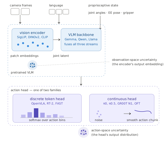
at a high level a VLA has three pieces. a vision encoder (typically siglip, dinov2 or a similar pretrained image backbone) turns raw camera frames into a sequence of patch embeddings. these embeddings, together with tokenized language instructions, feed into a backbone, almost always a pretrained LLM (qwen, llama, paligemma and variants). the backbone fuses vision and language into a joint latent representation conditioned on the task instruction. on top of the backbone sits an action head, which is the part that varies most across VLAs.

token output VLAs (openvla, rt2) discretize the action space into bins and treat each action dimension as a token in an autoregressive vocabulary. the action head here is a softmax over those discrete action tokens. continuous output VLAs (pi0, pi0.5, gr00t, openvla-oft) keep the action space continuous and use a generative head which is usually flow matching or diffusion, to sample chunks of actions from a learned distribution conditioned on the backbone’s output.

note: we’re moving towards continuous action spaces which handle multimodality and precision well. the discretised bins and autoregressive action chunks are older decoder methods not used anymore. i’ve added it here for completeness.

the observation side of the story is the same across both. the vision encoder gives the spatial signal. when a new image comes in thats outside the training distribution, the patch embeddings it produces drift away from the manifold the backbone was trained to consume. though we can sometimes catch this at the raw pixel level, the signal is much sharper at the embedding level because the encoder has already filtered out features that the policy is invariant to. observation space uncertainty methods sit on this embedding.

the action side depends on the head. for token output VLAs we can read the softmax distribution directly where high entropy over the action tokens means the policy is genuinely unsure between options whereas low entropy means it is confident. for discrete spaces where we can softmax and measure entropy loss, we have a lot of statistical tools to directly get uncertainty values. for continuous output VLAs there is no softmax to read as the action head produces a sample from an unnormalized density. the only way to surface uncertainty is to sample multiple chunks at the same observation and measure their disagreement, which captures multimodality the same way an entropy measurement would but costs more inference per timestep.

new observations and new actions disturb these representations differently. these two signals catch different things. imagine the camera sees a new object the encoder has never trained on. the patch embeddings drift into a region the backbone hasn’t seen, so observation side uncertainty spikes. but the policy can still confidently spit out an action chunk that just happens to be the wrong one, so action side uncertainty stays low. now lets flip it. imagine an arm stuck in a familiar scene, the camera image looks perfectly normal so the encoder is happy, but the policy doesn’t know how to recover so the sampled action chunks scatter or the token softmax goes flat. observation side stays correct but action side spikes. running just one of the two would miss whichever family the other catches, which is why we need to track both.

observation space techniques: RND-OE and SMD¶

two primitives anchor observation space novelty detection for VLAs. random network distillation(RND) on observation embeddings (RND-OE) and mahalanobis distance on the low dimensional state vector (SMD). they answer the same question, “has the observation moved off the manifold the policy was trained on”, but they operate at different layers of the stack and are also computationally complementary.

RND-OE. we spin up two small neural networks, identical input shape, m-dimensional output. one of them, we call it target, gets random initialization and is frozen forever. the other, call it the predictor, is trained to match the target’s output on in distribution(ID) data using straight MSE. the only thing the predictor can learn from this is to memorize what the random target outputs on the training inputs. think of it like a mapping function or a fixed random projection. so when you feed it a fresh input that looks like the training distribution, the predictor’s output is close to the target’s. but when we feed it an out of distribution(OOD) input and the predictor wasn’t trained on anything like it, the output diverges.

the score is just the residual,

$s_\text{RND}(x) = \| f_\theta(x) - g(x) \|^2$

where $g$ is the frozen target and $f_\theta$ is the trained predictor. the training loss is the same expression averaged over in-distribution samples, $\mathcal{L}(\theta) = \mathbb{E}_{x \sim \mathcal{D}_\text{ID}}\big[\| f_\theta(x) - g(x) \|^2\big]$. at inference, low residual means in-distribution, high residual means novel.

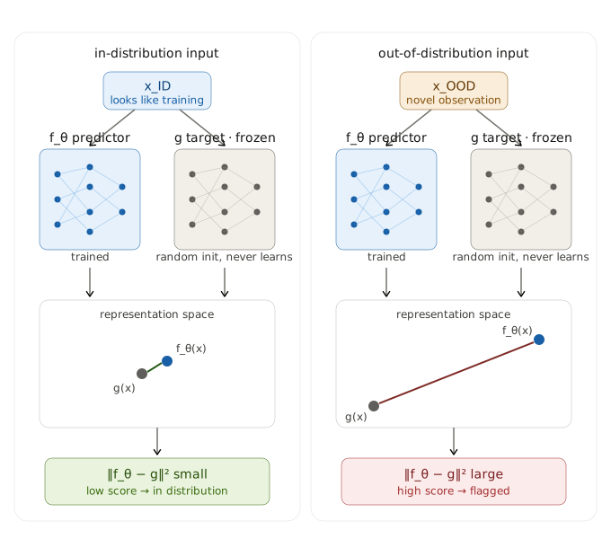
the construction was originally introduced for online RL (burda et al., 2018) as an exploration bonus, the agent gets rewarded for seeking out states where the residual is high because high residual means “i haven’t seen this before, go explore.” the same construction can be used for failure detection by flipping the sign of intent. instead of seeking high residual states, we threshold the residual and halt or hand off when it spikes. same network and same training but opposite downstream use. FIPER is the paper that applies this construction as the observation side scorer for VLAs.

the -OE suffix tells that the two network method we discussed, works on the observation space, which is the encoder output. we can run RND on raw pixels (RND-O) as well, but we get redundant information in pixels which we don’t really want to be comparing distribution shifts with. for eg, change the wallpaper color and RND-O starts screaming even though the policy doesn’t actually care. the encodings are sharper as the encoder has already squashed the cosmetic axes by virtue of being trained to produce action relevant features, so an OOD signal in the embedding correlates much more tightly with “this is going to make the policy go brr.”

the limitation is that RND-OE is an input only signal. it tells us the observation is novel, but nothing about whether the policy is producing a confident action or a confused one. a policy can be in distribution on the observation embedding and still produce a wrong action chunk for reasons RND-OE can’t see. that’s why we’ll pair it with an action space score later in the post.

SMD. RND-OE can handle high dimensional image representations while SMD handles the proprioceptive side which is usually lower dimension. the state vector for an arm based VLA is typically eight to twenty floats which include end-effector position, orientation, gripper state, joint angles, and any additional sensor information. we can fit a single gaussian to the distribution of these vectors over the training rollouts, mean $\mu$ and covariance $\Sigma$, and then score a fresh state by how far it is from $\mu$ in the geometry that $\Sigma$ defines. ReconVLA is the paper that applies this construction as an observation space failure detector on real robot VLA rollouts.

that geometry is the mahalanobis distance,

$D_M(x) = \sqrt{(x - \mu)^\top \Sigma^{-1} (x - \mu)}$

unpack what each piece does. $(x - \mu)$ is the offset from the training mean, a d-vector. $\Sigma^{-1}$ is the inverse covariance, the multivariate generalization of “divide by variance.” $(x-\mu)^\top \Sigma^{-1} (x - \mu)$ is a scalar that says how many covariance-corrected standard deviations the input is away from the mean.

to make $\Sigma$ concrete, in two dimensions it takes the form

$\Sigma = \begin{pmatrix} \sigma_x^2 & \sigma_{xy} \\ \sigma_{xy} & \sigma_y^2 \end{pmatrix}$

where $\sigma_x^2$ and $\sigma_y^2$ are the per-dimension variances sitting on the diagonal, and $\sigma_{xy}$ is the cross-dimension covariance sitting off the diagonal (symmetric, so the matrix has only three free numbers in 2D). those three numbers fully determine the shape of the constant-distance contours of $D_M$, and they’re the cleanest way to see why mahalanobis collapses into euclidean in some cases and stays tilted-elliptical in others.

the geometry is pretty interesting to look at.

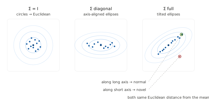
three sanity-check cases. when $\Sigma = I$, the inverse is also $I$ and the formula collapses to $\sqrt{(x-\mu)^\top (x-\mu)} = \|x - \mu\|$, plain euclidean distance with circular constant-distance contours. when $\Sigma$ is diagonal with unequal variances, the contours stretch into axis-aligned ellipses, dimensions with larger variance contribute less per unit deviation. when $\Sigma$ is full, with off-diagonal covariance terms, the contours rotate to align with the principal axes of the data cloud, correlated dimensions get treated as one effective axis. (see also arxiv 2305.13849 for related work on scoring gaussian-latent representations with mahalanobis.)

why this works on low-d state. covariance estimation needs sample size that scales with the number of parameters in $\Sigma$, which for d dimensions is $d(d+1)/2$. for an 8-D state vector with a few thousand training rollouts, you have plenty of data to fit 36 free parameters cleanly. it’s also free at inference, $\Sigma^{-1}$ is precomputed once, scoring a new state is one quadratic form, microseconds per timestep.

where it breaks. on a 768-D siglip embedding, $\Sigma$ has 295,296 unique numbers to estimate. a realistic training set has nowhere near enough samples to fit that many parameters reliably, so the fitted $\Sigma$ ends up with directions in the embedding space that look almost flat (very small estimated variance) just because not enough samples ever pushed along them. when we invert that covariance, those near flat directions explode in the inverse, and the mahalanobis distance loses meaning, tiny shifts in the input get scored as huge deviations. SMD therefore lives on the low dimensional proprioceptive state, while RND-OE lives on the high dimensional perception embedding. they don’t compete but instead cover different layers.

empirically SMD is shockingly effective. ReconVLA reports AUC 0.912 on real robot rollouts (UR5, 80 trajectories), beating every other detector they tested including RND variants and action instability heuristics. AUC of 0.912 means that if you pick a random failure rollout and a random successful rollout, the failure rollout scores higher 91% of the time. that means that SMD is creating a strong separation between successful and failed trajectories. to get this result with zero training and minimal compute is good, and makes SMD a good candidate to have as a detector.

these two together catch different failure families, the same observation vs action split from before but now playing out within the observation side itself. a novel object on a familiar arm fires RND-OE (the encoder produces an off-manifold embedding) but doesn’t fire SMD (the arm is in normal proprioceptive territory). a stuck arm in a familiar scene fires SMD (the joint angles are doing something the training distribution never saw) but doesn’t fire RND-OE (the camera sees a perfectly normal scene). running both in parallel gives you coverage of both at a combined inference cost that’s still trivial compared to the policy itself. that complementarity is why both make it into the proposal later.

action space techniques: ACE and quantile regression¶

the observation side detectors above tell us whether the input has moved off the training distribution. they don’t tell us anything about the distribution of the actions that the policy chunks out. for that we need to look at the action side of the architecture, specifically the action head outputs. there are two ways i found out people are doing it. action chunk entropy (ACE) for stochastic policies, and quantile regression for setting a calibrated bound on how far the policy’s action is from what an expert would have done.

action-chunk entropy (ACE). a stochastic policy (CVAE, diffusion or flow matching head) lets us sample multiple action chunks at the same observation, conditioning on the same state but creating fresh noise through the generative head each time. if the policy is confident about what to do, all the samples should land close to each other. if the policy is unsure (multiple strategies look plausible, or no strategy looks clearly right), the samples spread out or split into clusters. measuring that spread is the action side uncertainty signal.

honestly this took me a while to grasp so ill try being elaborate and intuitive while explaining how ACE works. the first idea to measure spread of any stochastic output would be to sample the output say B times, and then compute L2 variance. that turns out to be the wrong measure as a genuinely multimodal policy (say it’s equally happy grasping an object from the left or the right at this observation, both strategies succeed) produces two clusters of samples and therefore high L2 variance, even though the policy is not uncertain about what to do, it’s just that two different valid behaviors exist. variance conflates legitimate multimodality with confused spread so we need to have a better statistic to measure it.

we use entropy, which is a single number that measures how concentrated a probability distribution is across its possible outcomes. low when one outcome dominates and high when probability spreads evenly across many. for ACE, we take the B sampled action values at a single cell (one chunk step, one action dimension), bin them along the action axis into K bins, and treat the resulting bin counts as a probability histogram $p$ (we kinda try to discretise the continuous values each action outputs across the action dimensions). the shannon entropy of that histogram is $-\sum_k p_k \log p_k$, and it behaves in three distinct ways depending on what the policy did:

• confident: all B samples land in roughly one bin, the histogram has a single tall bar and everything else is near zero, entropy is low (close to 0).
• two legitimate modes: the B samples split into two clusters at separate bins (grasp left, grasp right), the histogram has two tall bars and everything else near zero, entropy is moderate (around $\log 2$ for two even modes).
• confused / no commitment: the B samples scatter across many bins, the histogram is roughly flat, entropy is high (approaching $\log K$ for fully uniform).

entropy therefore stays low when the policy is sure of itself, climbs to a moderate level when it’s juggling a few valid strategies, and spikes when it really doesn’t know what to do. L2 variance can’t make that distinction because the two cluster case and the random scatter case look equally spread out in terms of spatial distance.

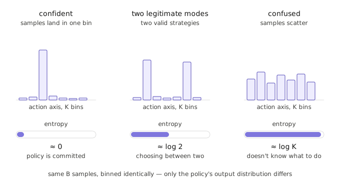
mechanically, at observation $O_t$ the policy outputs an action chunk $A_t \in \mathbb{R}^{H \times D}$ that plans $H$ timesteps ahead, each with $D$ action dimensions. we sample $B$ such chunks $\{A_t^{(1)}, A_t^{(2)}, \dots, A_t^{(B)}\}$ from the stochastic head at the same $O_t$, rolling fresh noise through the head each time. for each grid cell $(h, d)$ we collect the $B$ values at that cell across the samples, $\{A_t^{(b)}[h, d]\}_{b=1}^{B}$, bin them into $K$ bins to get a probability histogram $p_t^{(h,d)}$, and compute its Shannon entropy at that cell,

$H_t(h, d) = -\sum_{k=1}^{K} p_{t,k}^{(h,d)} \log p_{t,k}^{(h,d)}.$

the per observation ACE score is the sum of these per cell entropies across the whole grid,

$s_\text{ACE}(t) = \sum_{h=1}^{H} \sum_{d=1}^{D} H_t(h, d).$

we repeat this at every timestep $t$ of the rollout to get a stream of scores $s_\text{ACE}(0), s_\text{ACE}(1), s_\text{ACE}(2), \dots$ that we threshold the same way RND-OE and SMD were thresholded on the observation side. FIPER uses this construction as their action side scorer, paired with RND-OE on the observation side.

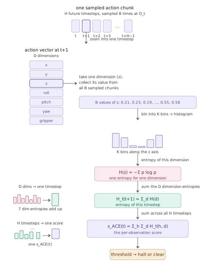
getting this action score is a bit computationally expensive though. B chunks at the same observation means B forward passes through the action head per timestep. for a flow matching head with 5-10 inference steps and B=32, that’s roughly 200 head passes per timestep. for a diffusion head at 100 inference steps and B=256, we have at 25k+ denoising steps per timestep, which is brutally slow for realtime use. the practical move is to create a tiered system where we use ace only when there is a pre-req signal which gets triggered.

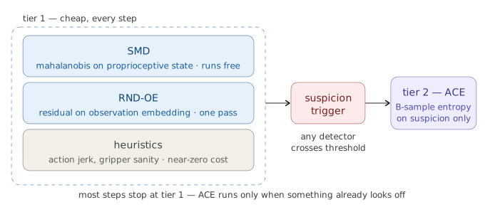
most of the time the cheap detectors don’t fire and we skip ACE entirely. but when the cheap detector trips, we can probably run ACE for a few timesteps to confirm the policy is actually confused before halting or handing off. the combined budget would stay small.

also to be noted that ACE only works on stochastic policies. for a deterministic policy (one observation, one action, no randomness in the head) ACE is meaningless, all B “samples” would be identical. for VLAs with a deterministic head (some of the earlier OpenVLA variants, action tokenized models run without temperature sampling) we need a different action side signal, which is where quantile regression comes in.

quantile regression (QR). standard regression with MSE loss recovers $\mathbb{E}[y \mid x]$, the conditional mean. sometimes we want a specific percentile of the conditional distribution instead of the mean, and that’s what quantile regression predicts. formally, if $F_{y\mid x}$ is the conditional CDF of $y$ given $x$, then the $\tau$-quantile is its inverse,

$\hat{q}_\tau(x) = F^{-1}_{y \mid x}(\tau), \quad \tau \in (0, 1),$

which reads as “the value of $y$ below which exactly fraction $\tau$ of the conditional distribution of $y$ sits.” $\tau = 0.5$ is the median, $\tau = 0.9$ is an upper bound that 90% of the values fall under, $\tau = 0.1$ is a lower bound that 90% of the values exceed.

to make this concrete in robot action space, imagine we want to predict where the gripper’s x coordinate should be at the next timestep, given the current state. now different expert demonstrations during training placed the gripper slightly differently at the same state, so the next gripper x position is a random variable conditional on the state. standard regression with MSE returns the mean of those expert positions. quantile regression at $\tau = 0.9$ instead returns the value such that 90% of the expert demonstrations placed the gripper below it, an upper bound on what counts as normal expert behavior at this state. if the policy’s actual action exceeds that bound at runtime, the action is operating in a regime that experts rarely went into, which is a useful uncertainty signal.

the loss that does this is the pinball loss,

$L_\tau(u) = \begin{cases} \tau \cdot u & u \geq 0 \\ (\tau - 1) \cdot u & u < 0 \end{cases}, \quad u = y_\text{true} - \hat{q}_\tau(x).$

it’s an asymmetric V. for $\tau = 0.9$, underestimating $y$ (predicted quantile is below the true value) costs $0.9 \cdot u$ per unit, while overestimating (predicted is above the true) costs $0.1 \cdot |u|$ per unit. the 9:1 imbalance pulls the predicted quantile upward during training until exactly 10% of training values sit above it, which is the definition of the 0.9 quantile. at $\tau = 0.5$ both arms become 0.5, the loss is symmetric (it reduces to MAE), and the predicted quantile is the median.

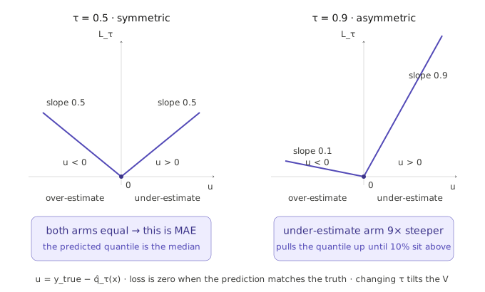
architecturally this is the same model as a regression network, just a different loss function. the output is now a calibrated percentile instead of a mean. on its own QR doesn’t guarantee that the predicted quantile matches the true quantile (it can be biased, capacity-limited, off because of distribution shift between train and deployment), but wrapping it with conformal prediction(CP) fixes that gap with a precision guarantee. even ACE benefits from CP as it is used to define thresholds for the scores.

conformal prediction: the calibration layer¶

every score we’ve discussed so far gives us a real number per timestep. RND-OE residual, mahalanobis distance, ACE entropy, QR percentile. all unitless scores that somewhat quantify uncertainty, but a raw number on its own doesn’t tell us when to actually halt the policy. to use any of these as a runtime alarm we need a threshold which tells at what value does the score cross from in distribution to failure prone territory. picking that threshold by hand is hard because the score has no obvious physical interpretation, and even a hand tuned threshold gives us no formal sense of how often it will misfire on real deployment data.

conformal prediction (CP) is an empirical method to pick the threshold with a concrete statistical guarantee attached to it. the idea is to set aside a separate batch of successful in distribution rollouts (we’ll call this the calibration set), run the score function on each of those rollouts, and use the distribution of scores observed on this set to fix the threshold. it gives a precision guarantee relative to the distribution that the calibration set was drawn from. this also means that the guarantee can break if the distribution of the policy changes (it is patched/finetuned/replaced). we will have to calibrate again.

to compute this threshold, we hold out a calibration set of $M$ successful in distribution rollouts, run our score function on each, get $M$ scores $s_1, s_2, \dots, s_M$, and take the empirical $(1-\delta)$ quantile of those scores as our threshold. on a fresh sample drawn independently from the same distribution as the calibration set (IID), the probability that its score exceeds the threshold is at most $\delta$.

from a mathematical perspective, the threshold is,

$\gamma = \inf\left\{ \beta : \frac{|\{i : s_i \le \beta\}|}{M} \ge \frac{\lceil(M+1)(1-\delta)\rceil}{M} \right\}$

read left to right, this says to walk up the score axis and stop at the smallest $\beta$ such that at least a $\lceil(M+1)(1-\delta)\rceil/M$ fraction of the calibration scores sit at or below it. that smallest $\beta$ is our threshold $\gamma$. it’s just the empirical $(1-\delta)$ quantile of the calibration scores, with a tiny upward nudge.

the $(M+1)$ in the numerator instead of $M$ is the finite sample correction, it accounts for the test sample’s own randomness and turns the guarantee into an honest IID coverage statement. $\delta$ is the miscoverage rate, a knob we choose, not a learned parameter. in failure detection language, $\delta$ is the false alarm rate we are willing to tolerate on successful rollouts.

CP guarantees that if calibration and test samples are independent and identically distributed(IID) , the false alarm rate on successful rollouts is at most $\delta$. that’s it. it does not guarantee anything about catching real failures. thats a recall question and recall depends entirely on whether the score function actually separates success from failure in the first place. CP just gives a precision guarantee.

we use forms of CP across the two uncertainty quantification techniques we discussed for the action space.

windowed max for ACE. the raw per step ACE score $s_\text{ACE}(t)$ is noisy. one bad chunk in a sequence of otherwise fine ones can spike the score even if the policy is fine on average over a few timesteps and a single spike triggering an alarm gives us a fragile detector. FIPER handles this by aggregating with a trailing sliding window of size $w$ before thresholding, taking the max over the window.

$\eta(t) = \max_{\tau \in [t-w+1,\, t]} s_\text{ACE}(\tau).$

then $\eta(t)$ is the quantity that gets thresholded against the CP-calibrated $\gamma$.

for the sliding window that we roll across the trajectory, we could have also averaged out values to reduce spikes, or summed values to preserve temporal context in scores, but sum would scale with $w$ (a longer window mechanically yields a bigger number), so the threshold would have to be recalibrated for every window size we try, which is brittle. mean would be scale invariant but would miss out on genuine spikes (one bad chunk in a window of 20 fine ones gets divided by 20, hiding the alarm signal). max preserves spikes and keeps the aggregated score on the same scale as the raw per step score. the CP threshold stays stable as we vary $w$. this was discussed more in the FIPER paper if you want to dig deeper.

CQR: CP wrapped around QR. quantile regression alone gives a predicted $\tau$-quantile, but does not guarantee that prediction matches the true $\tau$-quantile. we don’t know if the model is biased, is mismatched from the policy as the policy might have updated, or is in general just not accurate with the true quantile. CP fixes that gap with one extra pass over a calibration set.

we train the QR model with the pinball loss discussed earlier to get $f_\tau(x)$. hold out a calibration set, and compute a conformity score on each example,

$S_j = y_j - f_\tau(x_j),$

(positive $S_j$ means QR underestimated the $\tau$-quantile on this sample). take the $(1-\alpha)$ quantile of $\{S_j\}_{j=1}^M$ as the calibration offset $q_\tau$. the calibrated upper bound then becomes $f_\tau(x) + q_\tau$

$P\big(y_\text{new} \le f_\tau(x_\text{new}) + q_\tau\big) \ge 1 - \alpha.$

$\alpha$ here plays the same role $\delta$ did earlier, the miscoverage rate we are willing to tolerate, a knob we choose. setting $\alpha = 0.1$ means we want the calibrated bound to cover the true value at least 90% of the time on fresh IID samples.

this is standard conformal prediction applied to a regression bound instead of an anomaly score. and it gives us a calibrated number we can score candidate actions against, which is exactly how ReconVLA uses CQR for action selection out of $B$ candidates sampled from a stochastic policy.

also note that RND-OE, SMD, ACE were framed as alarms where we run the score and compare against a threshold to detect uncertainty that can lead to failure. in a lot of the papers, action space techniques like ACE and CQR have also been proposed as action selectors for inference. sample $B$ candidate chunks from the stochastic policy at the same timestep, score each one, and instead of executing the first sample, execute the one with the lowest uncertainty. the policy stays exactly as it was but we just bias its sampling toward the safer of the candidates it itself produced. ACE does this by scoring each candidate against the spread of the $B$ samples and keeping the one that sits in the densest, lowest entropy region rather than an outlier mode, CQR does it by picking the chunk whose predicted action sits closest to the calibrated bound on expert behavior.

another thing to note is a limitation of CQR and how calibration isn’t really a holy grail of a solution for everything when the intrinsic failure scoring itself has weaknesses. for example, CQR’s score is ‘distance from what an expert would have done’ at a given state. that is a perfectly valid signal when the task has one correct strategy. but when the task is multimodal (multiple valid strategies exist) distance from expert, isn’t a strong enough metric to gauge probability of failure because another mode of trajectory might be deviating from the expert but still lead to task success.

ReconVLA found CQR improved most of their tasks as an action selector, but on tasks where valid behaviors deviated sharply from the expert it struggled. their milk task is the clearest example. there were two legitimate ways to grasp the carton, a side grasp (mode A, what the expert demos showed) and a top grasp (mode B, what the policy sometimes prefers based on the observation). both succeed when executed but CQR was trained against Mode A expert demos, so at runtime it scores Mode B candidates as high uncertainty and filters them out. with CQR turned on as the action selector on this task, the success rate drops from 60% to 47% because the policy gets forced into Mode A even on observations where Mode B was the better fit. the flow matching head produced the multimodality (its a good thing as it captured the policy’s actual options) but CQR’s training signal collapsed it (a bad thing, it treated a valid alternative as out of distribution).

calibration didn’t break here, but the underlying signal was the problem. CQR is calibrated to the distance-from-expert distribution, it is not calibrated to the failure distribution. so though calibration is important, improving the scoring function becomes first priority here.

this also reinforces the architectural idea that action side uncertainty needs an intrinsic signal (policy disagreement with itself, like ACE) rather than an extrinsic signal (deviation from a single expert, like CQR), or it needs multi expert training data to actually cover the multimodality. the cleanest pattern is to use CQR carefully in regions where the task is genuinely unimodal, and lean on ACE in regions where multiple strategies are valid. i will reiterate on this in my proposed architecture

adding temporality to uncertainty¶

while i was synthesising notes on uncertainty quantification from the papers i had read, i came across a recent twitter post on TDQC, a recent ICML 2026 accept that added a new lens to the whole problem in a way i hadn’t been thinking about. all the techniques discussed so far calibrate a single score at a single timestep, RND-OE on the current observation, ACE on the current action chunk, CQR on the current candidate action. TDQC(Temporal Difference Calibration in Sequential Tasks) pushes calibration into the time axis. instead of asking “is this timestep weird” it asks “given everything we have seen up to this point in the rollout, what is the probability the rollout eventually succeeds.” this framing and the loss looks identical to a temporal difference loss from RL shaped as Q learning. the predictor itself IS a value function. i spent a while digging through the paper and in a nutshell, TDQC trains a small head $f_\theta(h_t)$ on the policy’s running history $h_t$ (the sequence of observations and actions so far) to predict $P(\text{success} \mid h_t)$. the loss they use during training is a sequential variant of the brier score, which is just mean squared error between the predicted probability and the eventual binary outcome $y \in \{0, 1\}$,

$\mathcal{L}_\text{Brier}(f, t) = \mathbb{E}\big[(f(h_t) - y)^2\big].$

training against this loss leads to a function that minimizes MSE against a binary target and is the conditional expectation:

$f^*(h_t) = \mathbb{E}[y \mid h_t].$

if $y$ is the binary success indicator at the end of the rollout, $\mathbb{E}[y \mid h_t]$ is the probability of eventual success conditioned on the history so far. but $\mathbb{E}[y \mid h_t]$ under a fixed policy $\pi$ is also exactly the definition of the value function $V^\pi(h_t)$ from RL, the expected return under $\pi$ given the current state. so calibrated success probability and the policy’s value function are essentially the same mathematical object viewed differently across fields. this also means the training procedure can be borrowed from RL. the loss term only ever sees the terminal $y$, so every $h_t$ along the trajectory gets supervised by the same scalar regardless of how close it is to the outcome. the temporal structure between $h_t$ and $h_{t+1}$ is missing. temporal difference(TD) learning fixes this by using the next step’s prediction as a soft target for the current step, so every transition carries gradient signal, not just the terminal one,

$\mathcal{L}_\text{TD}(\theta) = \sum_t \big(f_\theta(h_t) - f_{\theta^-}(h_{t+1})\big)^2 + \text{terminal anchor on } y.$

the $\theta^-$ is a target network, a frozen slowly updating copy of $\theta$ (from DQNs) (mnih et al., 2015). without it, both sides of the squared error move at every gradient step (because $f_\theta$ on the left and on the right share parameters), the target chases its own tail and training oscillates. freezing the right hand side for $C$ steps at a time gives the left hand side a stationary target to fit against, and you periodically refresh the freeze. its a pretty standard method we also see in Q learning

so we can derive two things from TDQC for our failure detection architecture. one, a calibrated $P(\text{success} \mid h_t)$ at every timestep. threshold it below some value and we can have an early stopping signal that fires when the rollout is statistically unlikely to succeed, even before anything visibly goes wrong. second, the score works on action probabilities alone (a variant they call RNN-TDQC), which means we don’t need access to the policy’s internal activation like other methods. this matters because in the real deployment world, customers running closed source VLAs (API served policies, future commercial models) can still get a calibrated failure signal without ever accessing weights or hidden states.

beyond detection, since $f_\theta \approx V^\pi$, the same head also gives us an advantage signal,

$A_t = f_\theta(h_{t+1}) - f_\theta(h_t),$

which is continuous even though the underlying success label is binary, because $f_\theta$ produces a smooth probability. this can create an actor critic loop for the policy where the VLA is the actor, $f_\theta$ is the critic, advantage is the gradient signal that tells us which actions to upweight. we detect failures with $f_\theta$, then use the same $f_\theta$ to nudge the policy in the right direction. this is just one of the ways we can extend detection into resolving errors, but we will talk more about resolution in future blog posts. just a point to be noted here is that the same primitive that closes the alarm loop also opens the door to the patch loop, which is exactly the bridges i need to research and scope for the broader self improving robots architecture i am working towards.

a fine tuned VLM judge at the top of the detectors¶

the techniques discussed so far are all high frequency, cheaply computed signals which sit alongside the policy without interfering with the inference loop. there is also a separate line of research on using VLMs directly to analyze trajectories and errors. running a VLM at every step is not realistic as the latency hit on the control loop is too large, but it doesn’t have to run every step. an async system that runs a VLM every $N$ steps, or only when the cheaper detectors below it have already raised a flag, seems like the right way to build it.

FailSafe is the clearest example of this. they fine tune LLaVA-OneVision-7B into a failure aware visual judge that, given the current observation and a short window of recent frames, classifies what kind of failure is happening. the interesting thing about a fine tuned VLM at this tier is that it doesn’t just produce a binary alarm but also a label (slipped grasp, wrong object, stalled motion, no-op loop, etc). qualitatively identifying the failure mode is a different kind of signal than the scalar scores from the lower tiers, it tells us not just that something is wrong but what caused the failure, which is what we will eventually want when we move into isolating and patching failures. FailSafe also goes one step further and emits an executable $\Delta$-action that another VLA can consume as a recovery nudge, which is correction not detection, and lives in a separate block of research i’m doing. i will pull on that separately when i scope and write about failure to correction loops. for failure identification, what we can take from FailSafe is the classification head, the tiered pattern, and the architectural shape of a slow expensive judge sitting on top of cheap detectors.

composing these methods into a deployable system¶

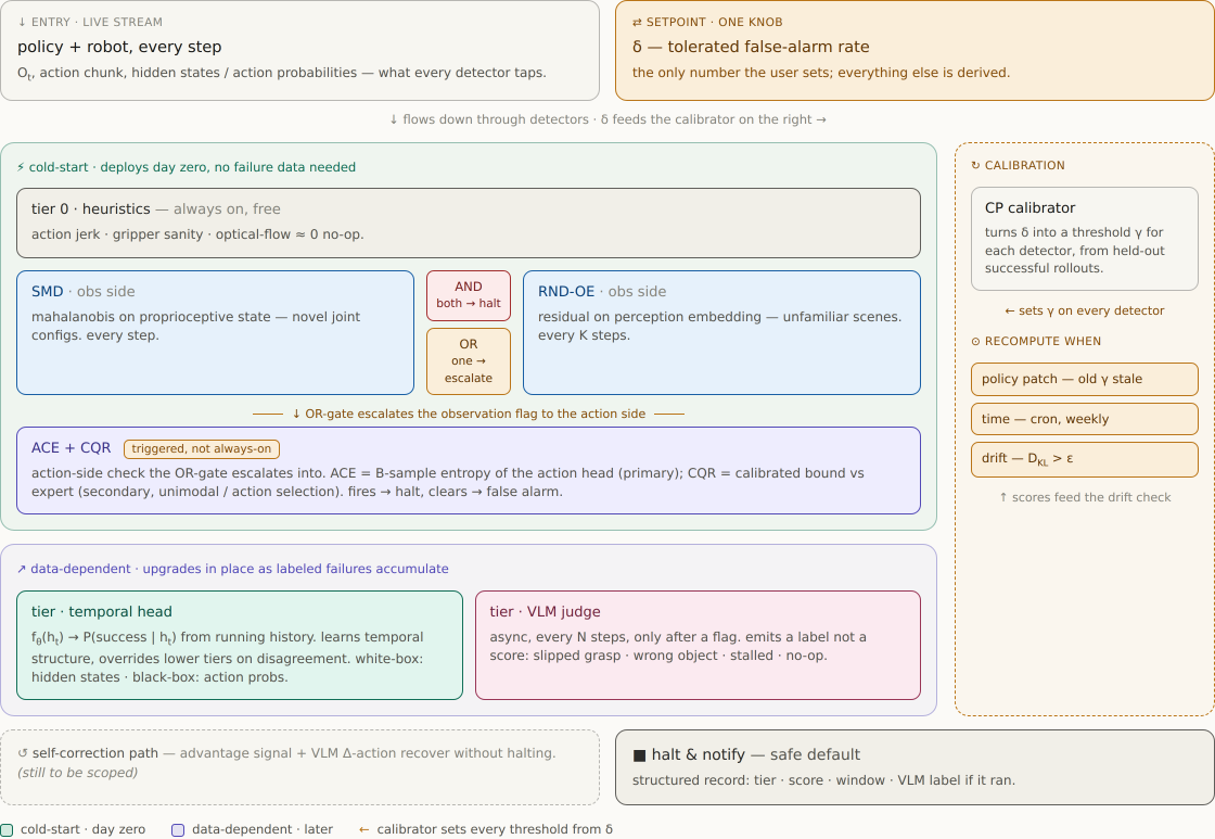
every primitive in this post has been validated on benchmarks in isolation, RND-OE on FIPER, SMD and CQR on ReconVLA, ACE on FIPER, TDQC on its own ICML benchmarks, FailSafe on ManiSkill. what doesn’t exist in the published work yet is a single cohesive system that composes multiple of these techniques into something production ready. it would give the user one knob to turn, autocalibrate according to the distribution of the policy, and take care of chaining and cascaded validation through a number of UQ techniques. i tried sketching what a composition of such a system looks like.

a few things i’m trying to keep true across the design. the stack should be deployable without any prior failure data, which means the methods that depend on failure data (TDQC, fine tuned VLM judges) come online later once flagged trajectories have accumulated. the user should only see one knob, something like “alarm me when failure probability exceeds 5%”, and the architecture translates that internally into per primitive thresholds and recalibration cadence. it should work across both discrete token output VLAs (OpenVLA, rt2) and continuous output VLAs (pi0, pi0.5, OpenVLA-OFT, etc), and it should degrade gracefully from the white box case (we own the policy weights) to the black box case (we’re querying an API served closed source policy). and recalibration has to be automatic, because conformal prediction will break every time the policy is patched, environment expands to a newer task space, or the customer site shifts.

cascading tiers¶

the cheap tiers run at every step alongside the policy, the expensive ones only run when something below them has already raised a flag. each tier targets a different question which expands the coverage/kinds of uncertainty we’re catering to

the cheapest layer should be a set of classical heuristics which might be jerk thresholds on actuator commands, gripper state sanity checks, wrist cam optical flow near zero as a no-op detector. these cost nothing and ReconVLA’s tables show they’re more competitive than learned detectors on old VLA generations

the next layer will be the observation side, where SMD on the proprioceptive state and RND-OE on the perception embedding run in parallel. SMD doesn’t add compute so it can essentially run every step. RND-OE is a forward pass through the predictor and a residual computation which makes it a bit more expensive, so it runs less often, say every $K=5$ steps or whenever SMD has already flagged something. they’re both observation side but catch different things, SMD catches “the robot is in a joint configuration the demos never showed,” RND-OE catches “the scene looks unfamiliar to the encoder.” when both fire at the same step that’s a strong joint signal and we halt directly. when only one fires, the architecture doesn’t trust the cheap signal on its own and escalates to the action side instead.

the action side, when triggered, runs ACE. we sample $B$ chunks from the stochastic head at the current observation, compute per cell Shannon entropy across the $B$ samples, aggregate with the trailing windowed max we talked about earlier and threshold against the CP calibrated $\gamma$. if ACE fires we halt, if it clears, we treat the observation side trigger as a false alarm and continue. CQR sits parallel to ACE as a secondary score, useful on tasks that are unimodal or where we have multi expert demos to train it across the legitimate modes. i’d keep ACE as the primary action side alarm in v0 because CQR’s failure mode is silent, we don’t get warned on the tasks where it’s hurting performance rather than helping.

once we’ve accumulated enough labeled failures from the lower tiers, we can also use a temporal network for failure prediction. once trained, it produces a calibrated $P(\text{success} \mid h_t)$ at every step from the running history, which is a stricter signal than the windowed max because it actually learns the temporal structure rather than aggregating over it. when this tier is up, it can override the lower tiers on disagreement, because its signal is the only one calibrated to the actual success distribution rather than to an indirect proxy.

the top or highest level of the detection would be a slow moving subsystem. a fine tuned VLM judge, triggered when any of the lower tiers has already flagged something, and running every $N$ steps async so the control loop never waits on it. though it will periodically be used to do sanity checks on the downstream detectors, its job will be more around producing labels like ‘slipped grasp’, ‘wrong object’, ‘stalled motion’, ‘no-op’. These categorical signals will later be useful for failure attribution and corrections. (we will talk about that in a separate post)

handling different VLA architectures¶

the tiers and configuration of the detection system should be able to dynamically change according to the policy architecture. on a continuous head policy like pi0.5, the flow matching head doesn’t expose a probability distribution we can read off, so ACE has to go through the full $B$-sample then bin then entropy path from before, the histogram is how we discretize the continuous samples into something Shannon entropy is even defined on. CQR runs on a regression bound. on a discrete token head policy like OpenVLA, the softmax over action tokens is already a discrete distribution, so ACE can skip the sampling step and read entropy off the softmax directly. when we have white box access we run detection on hidden states, when we don’t we fall back to working with action probabilities alone. the system should be generalisable enough to cater to these differences

a single hyperparameter should be enough to create thresholds¶

conformal prediction as a term shouldn’t be cared for by the end user setting the threshold/monitor. the user sets one number, the global false alarm rate $\delta$ they’re willing to tolerate on successful rollouts, and the architecture translates that into per primitive thresholds. each primitive gets its own CP calibration against its own held out successful rollouts. for the cheap observation tier where two primitives are AND combined, $\delta$ has to be allocated across the two so that the joint false alarm rate stays under the user’s target, and that allocation is one of the open questions because marginal CP guarantees don’t automatically compose into joint guarantees. for temporal calibration, $\delta$ becomes the threshold on $1 - f_\theta(h_t)$ directly because the head is already calibrated to outcome probability. the user never sees $\gamma$, $q_\tau$, window sizes, or any of the internal hyperparameters, they see a single knob and the architecture should handle the translation.

how the calibration actually happens¶

the IID assumption that gives CP its guarantee can break because of changes in the policy or the world. the autocalibration architecture should have multiple ways to to identify drift and calibrate. we can add a few rules to make this robust. one, calibration is patch driven, every time the policy gets updated, fine tuned, or replaced, every learned primitive’s calibration set is stale, because the score distribution was fit to the old policy. recalibration has to run on a fresh batch of successful rollouts from the new policy before deployment resumes. the second is time driven, even with no policy update the world drifts, lighting shifts, object wear, the customer reconfigures the workspace. so the architecture keeps a rolling buffer of the last few days of successful rollouts and recomputes thresholds on a cadence, weekly is a reasonable default. the third is drift driven, the architecture continuously monitors the score distribution on running rollouts and compares against the distribution at the time of the last calibration.

written down, this is just calling $P_\text{cal}$ the histogram of scores we saw on the calibration set the last time we recalibrated, and $P_t$ the histogram of scores over the most recent rolling window of length $w$ of successful rollouts. KL divergence then becomes

$D_\text{KL}(P_t \| P_\text{cal}) = \sum_i P_t(i) \log \frac{P_t(i)}{P_\text{cal}(i)},$

we trigger a recalibration when $D_\text{KL}(P_t \| P_\text{cal}) > \epsilon$ for some small tolerance $\epsilon$ that the system holds. intuitively, $P_t$ is what the world is producing now, $P_\text{cal}$ is what the world was producing when we last calibrated, and the KL is asking how surprised the calibration distribution would be by the current one. small KL means the two distributions are close enough that the existing threshold is still trustworthy. once KL crosses $\epsilon$, the calibration set has drifted out from under us and the cron schedule is too slow to catch it, so we recalibrate now instead of waiting for the weekly tick. the same trick works with other divergences but KL is the cheapest to compute on histograms.

the earliest version of this would probably just ship patch driven and time driven, both are cheap. drift driven needs more thought

starting without failure signals before using the data flywheel¶

initially, only the primitives requiring no failure data should be used(ACE,RND,SMD). once enough expert demos and failure trajectories get recorded, we can use networks trained with failure data, specially in the action space. every alarm gets logged with the full trajectory and structured metadata (which tier fired, what score, what window). a human (or eventually a replay based offline verifier) confirms or rejects each proposal, and confirmed failures pile up in a labeled dataset. the evolution of the tiered detection system, which adds temporal value estimation and VLM judge as and when the collected data increases, is automatic and not human touched.

the two output paths¶

once an alarm fires, the architecture has two possible downstream actions. one is the halt-and-notify path, where the policy stops, the operator gets the structured failure record with the tier, the score, the window, and the VLM’s label if it ran. this is the safer default and it’s how software systems have handled production alarms for decades. the second path is self correction, where the advantage signal and a VLM’s possible $\Delta$-action output drive a recovery without halting. that’s an extension to this post and something i’m going to research after this.

wrapping up, what comes next¶

most of what i’ve put down here is opinion shaped by facing the pain of not being able to get my robot trajectories to halt at failure, reading papers, and going down rabbit holes around failure detection. so before i actually implement a version of this architecture on a real robot, this will remain more a theoretical proposal than a proven production ready system. in a nutshell, a reliable failure detection system will have cheap observation side detectors running at every step, expensive action side ones only when the cheap layer has already flagged something, a temporal head that comes online once we’ve accumulated failure data, and a VLM judge at the top for labels. all of it wrapped in a calibration layer the user sees as one knob, with autocalibration that fires when the policy gets patched or the score distribution drifts.

now the actual implementation of such a system is still to be figured out, which would surface its own set of questions like how to allocate a single user facing $\delta$ across combined detectors without losing the precision guarantee, or how to turn continuous action samples into a discretised distribution we can compute entropy on, etc

on a broader level, this whole system is just the first step toward self improving robot policies that learn from their own failures in the field. once we can confidently identify when the policy is failing, the next pieces are isolating what caused the failure and using that signal to improve the model without retraining from scratch. each of which, require their own dedicated research sprints. the next thing for me personally is to take this architecture and try replicating it on my so-101 setup, a cheap 6 servo arm i’ve recently setup. i will start with the cheap detectors, calibrate on a small batch of successful rollouts, and see whether the precision/recall numbers come anywhere close to what the papers reported. i will then gradually extend and test the entire system on the arm.